Model comparison · field data
Which learning dynamic reproduces the crowd?
Eight population-level models fit to 49 days of the Swedish LUPI lottery. The winner isn’t decided by who predicts tomorrow best — it’s decided by whose free-running trajectory tracks reality.
The game
In LUPI (“Limbo”) each player picks an integer in
1–99,999; the lowest number chosen by exactly one
person wins. Players never learn how many others are playing (modelled
as Poisson with mean n), and the only public feedback is the daily
winning number. The data are one file per day, 49 rounds from January 2007.
Every anchor from the benchmark paper’s Table 1 reproduces exactly:
| Day 2007-01-29 — total / winner / lowest unplayed | 41,067 / 280 / 480 |
| Daily totals range | [38,933, 69,830] |
| Winning numbers range | [162, 4,465] |
| Grand average of chosen numbers | 2,835 |
| Mean daily bets (= the Poisson n) | 53,783 |
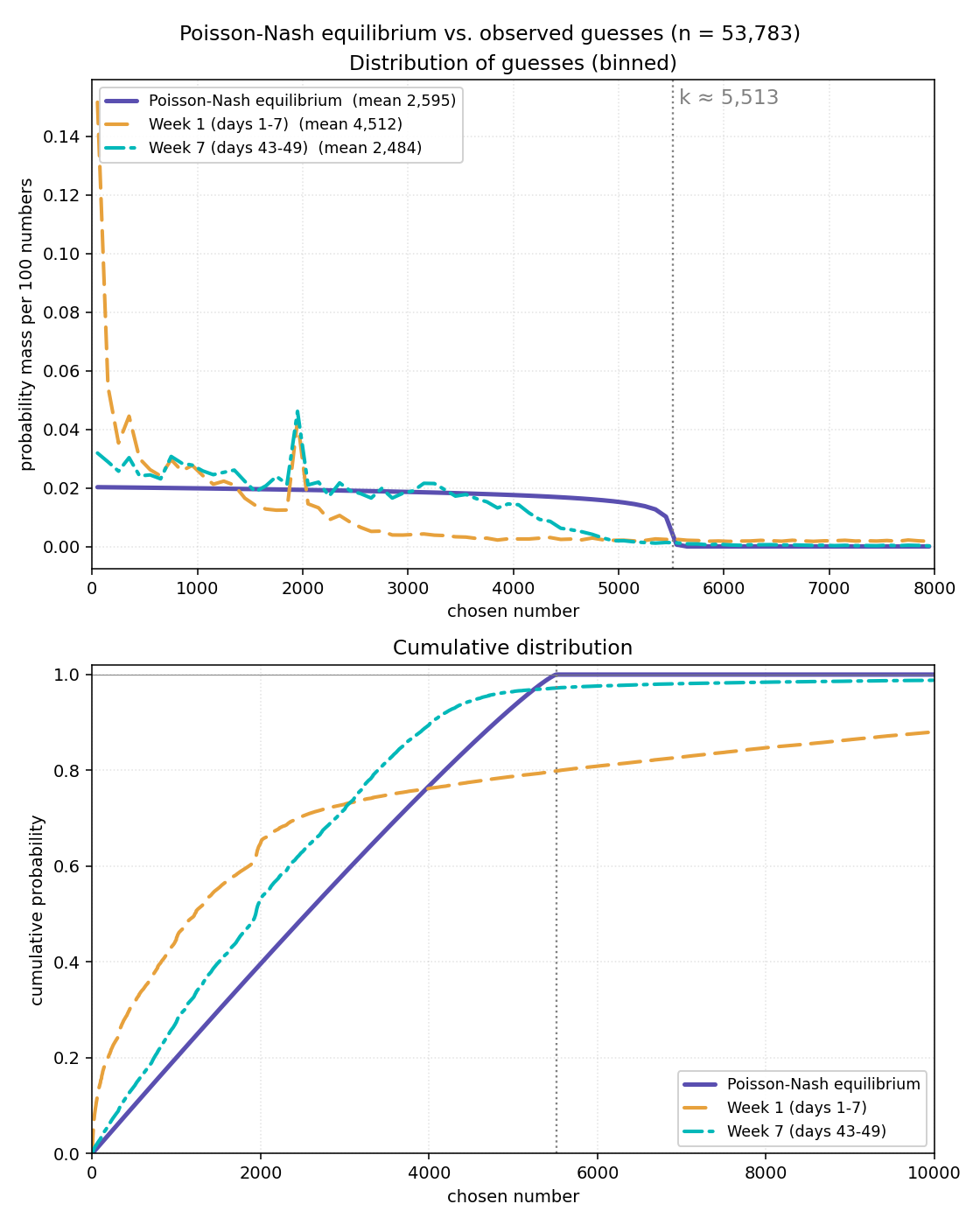
One fact drives everything: over the seven weeks the mean guess falls from 6,752 to ~2,400 and the mass on high numbers (above 5,513) collapses from 30% to ~3%. The crowd adapts toward the equilibrium region. Reproducing that adaptation is the models’ job.
The equilibrium is where they’re heading
Poisson–Nash, solved via the paper’s recurrence in intensities qₖ = n·pₖ
with the one free constant pinned by Σqₖ = n. It reproduces the paper’s implied mean of 2,595, support ending at 5,518, and payoff indifference across the support to machine precision. Week 1 sits far above it with a fat tail; by week 7 the crowd has collapsed onto it.
The contenders
Eight models sit in the standings below — three baselines that set the scale, and five learning models, each a different theory of how a player changes their number from one day to the next.
The baselines don’t learn; they mark the scale. Uniform spreads its bets evenly across all 99,999 numbers — the floor every real model must clear. Static Nash plays the equilibrium above, unchanged every day: it shows where the crowd is heading, not how it gets there. Persistence just replays yesterday’s distribution — “tomorrow = today” — a surprisingly strong one-day forecaster that, by construction, learns nothing.
Similarity-weighted imitation (the Mohlin–Östling–Wang benchmark) is copy what wins. After each round the winning number — and, through a triangular “close-enough” window, the numbers near it — gain a little attractiveness, and that pull accumulates over every past round; players then pick in proportion to accumulated attractiveness. No reasoning about opponents or payoffs, just imitation of recent winners and their neighbours. Because the whole crowd imitates together, the population slides toward the winning region fast.
Directional learning asks even less of a player: nudge your own number toward the last winner. Sat above it? A cheaper number won, so shade down. Sat below it? You were in the crowd that collided, so edge up. Only the direction matters — never the size of the gap or any payoff — and a dose of randomness plus differing step sizes keeps the crowd spread out instead of collapsing onto a single number.
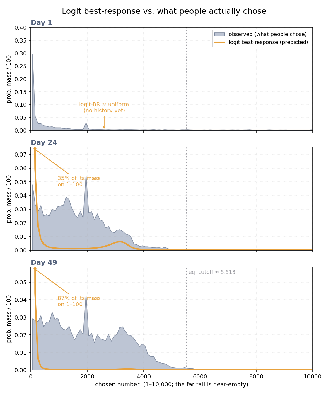
Logit best-response is the “rational” contender. A player forms a belief about where the crowd will be — a recency-weighted average of the whole past distribution — works out which numbers would most likely win against that crowd, and leans toward them (softly, because in LUPI wide bands of numbers are near-ties). The trap: since the winner is the lowest unique bet, its best reply is to undercut to the very smallest numbers — it ends up telling almost everyone to “play 1”, nothing like the spread-out real crowd.
Erev–Roth reinforcement is imitation with one ingredient removed: reinforce only what you did, not what the crowd did. But exactly one bet wins each day (the lowest unique one), so only that single player learns anything while everyone else stands pat — averaged over ~53,000 players, almost no movement at all, and the population stays frozen near its starting point. It is here to show precisely what imitation’s “copy the whole crowd’s success” step buys.
Experience-weighted attraction (EWA) is the umbrella that holds
reinforcement and belief-learning as the two ends of one dial. Every number k
carries an attraction Aₖ. Each day it is nudged by that
number’s foregone payoff πₖ — the win-probability it
would have earned against that day’s whole crowd — and the next day’s
play is a softmax over the attractions:
Four knobs steer it: δ is the dial — at δ = 0
only the number you actually played is credited (pure reinforcement), at δ = 1
every number is credited by its would-be payoff (belief-learning); φ sets
how fast old attractions fade; ρ sets how fast the experience count
N grows, which just turns the update into a running average; and
λ sets how sharply the softmax concentrates on the best-looking
numbers. Here fₖ is the fraction of the crowd that played k (the
population stand-in for “did I play k?”). All four are fit to the data by
maximum likelihood; where they land, and what they do to the curve, is in the Results below.
Seeing the disagreement
The standings below reduce each model to a single number. To make one concrete, here is the logit best-response model’s predicted distribution (amber line) laid over what people actually chose (shaded), for an early day, a middle day, and a late one. Everything is truncated to 1–10,000, where nearly all the mass sits; the far tail is near-empty and would only add whitespace.
Two ways to be right
The task. Each day, roughly 53,783 bets land somewhere on the numbers 1–99,999, and that day’s empirical distribution is simply the fraction of bets that went to each number. A model, fed the history so far, outputs its own predicted distribution over those numbers for the day. Being accurate means one thing: how close is the model’s predicted distribution to the one people actually produced? We measure that closeness in two ways.
Metric 1 — one-step-ahead. Each day, hand the model everything
that actually happened up to yesterday and ask: what is your distribution for today?
Then look at what people truly chose today, and score how much probability the model
had placed on those real choices. That score is the likelihood —
high when the model gave lots of probability to what actually happened, low when reality
caught it by surprise. Written out, it sums over every number k the
day’s bet count cₖ times the log of the probability
pₖ the model gave that number:
The log turns “multiply the probabilities of all 53,783 choices” into a sum, and weighting each number by how many people picked it lets popular numbers count for more. (We report the total per bet — in nats, the natural-log unit — so busy days don’t dominate; higher is better.)
Metric 2 — free-running rollout. Now give the model only
day 1, then make it generate day 2 from its own day-1 prediction, day 3
from its own day-2, and so on — 49 days entirely self-propelled, never shown real
data again. Then compare its self-generated trajectory to the actual one, day by day.
This is far harder, because small errors compound. We score each day’s gap with the
KL divergence, which in plain terms asks: if you were expecting the
model’s distribution but reality kept drawing from the actual one, how surprised
would you be on average? It sums over every number the real probability
qₖ times the log of how much more (or less) likely that number really
was than the model expected:
Zero means the two distributions are identical; the bigger it grows, the further apart they are (lower is better). Measuring surprise from reality’s side rather than the model’s is exactly what makes putting almost no probability where the crowd actually is so costly — the signature failure of the payoff-based models.
Two views of one ruler. The two metrics are close cousins: mathematically, minimising a day’s KL gap is almost the same as maximising its likelihood — just written as an average surprise per choice rather than a total. What really differs is the test. Metric 1 lets the model lean on reality every day; Metric 2 makes it stand on its own for seven weeks.
The standings
| Model | One-step LL / bet | Rollout KL | Verdict |
|---|---|---|---|
| Similarity-weighted imitationMohlin–Östling–Wang (MOW) | −8.60 | 0.40 | best rollout ★ |
| Directional learningagent anchors; collapses to smoothed persistence | −8.53 | 1.03 | best one-step |
| Static Nashthe equilibrium, played every day | −9.43 | 1.24 | the attractor |
| Erev–Rothown-experience reinforcement | −10.74 | 2.48 | fails: freezes |
| Logit best-responsebest-respond to the full crowd (Tier 3) | −10.53 | 2.48 | fails: plays 1 |
| Persistencetomorrow = today | −8.63 | 2.58 | short-run only |
| EWAexperience-weighted attraction | −11.27 | 2.91 | fails: spike / flood |
| Uniformthe floor | −11.32 | 3.08 | baseline |
Sorted by rollout KL (lower is better). Higher one-step LL/bet is better; the best value in each column is highlighted.
Results
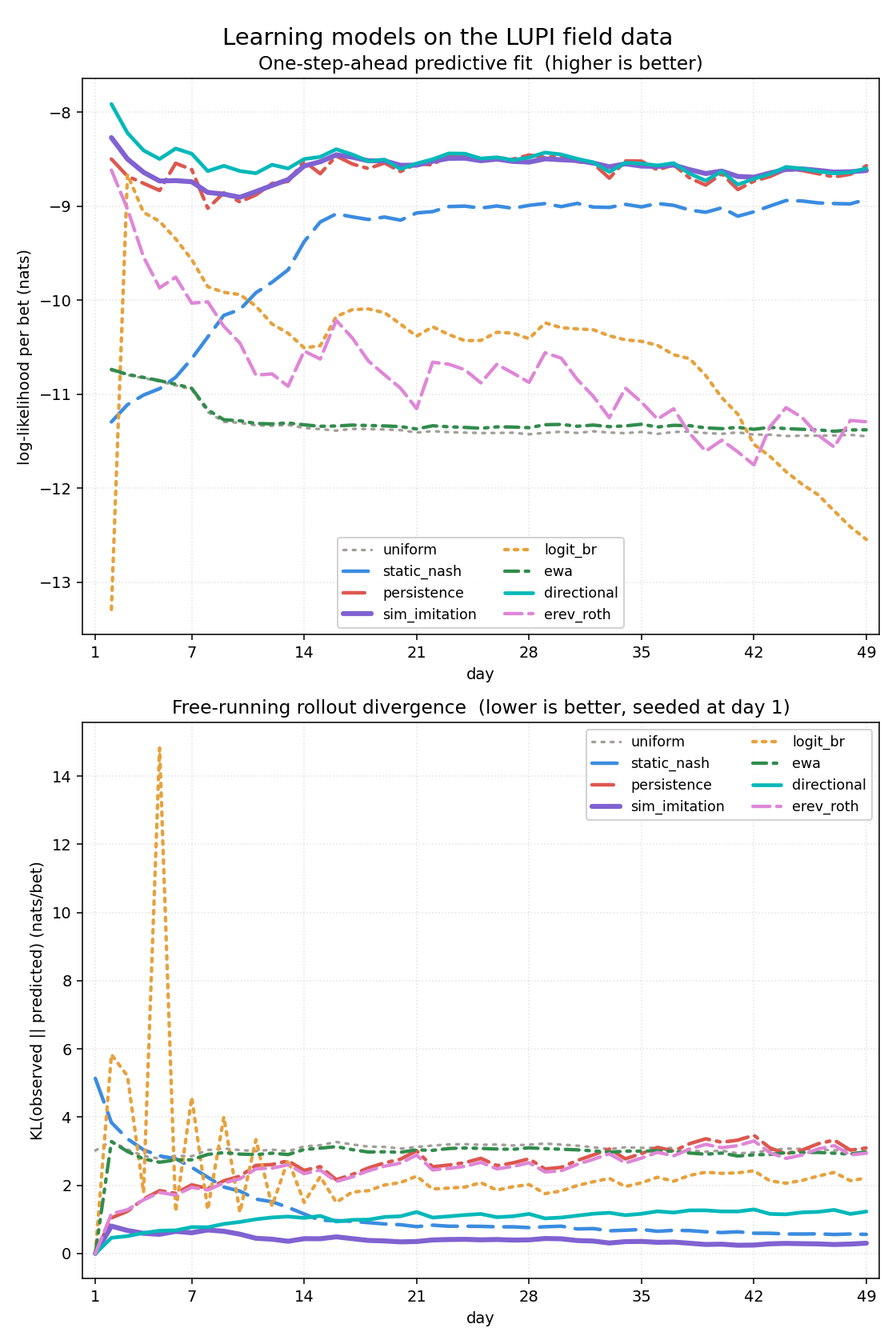
The standings compress each model to two numbers. Here is the fuller picture, model by model — the parameters each fit settled on, and why its one-step curve (higher is better) and free-running rollout (lower is better) trace the shapes they do. One thread runs through all of them: the same crowd that opens far above equilibrium and slides onto it over seven weeks is what animates every curve, and a model’s fate turns on whether it moves with the crowd or stands still.
Uniform. No parameters — a flat 1/99,999 every day, the
level-0 floor. Its one-step score isn’t quite constant, though, because the scorer
groups the sparse region above 10,000 into 500-wide bins, which makes a bet in the empty
tail read ~6.2 nats “cheaper” than one on a specific low number; uniform’s
per-bet score is therefore exactly log(1/K) plus 6.2 times the fraction of
bets above 10,000. As the crowd concentrates and that fraction collapses (12% on day 2
to 1% by day 49) the free lift evaporates and the curve sags from −10.7 toward
its floor of −11.5. Its rollout sits flat and worst-of-all near 3.08: a distribution
that never moves can never follow a crowd that does — and being literally chance, it
approaches that floor from above but never dips below it.
Static Nash. Also parameter-free: the equilibrium is solved once (implied mean 2,595, support ending at 5,518) and replayed unchanged, so again only the data moves. One-step starts at the uniform floor (−11.3 on day 2) and climbs steeply to a −8.9 to −9.1 plateau — early on a fifth of bets land above the equilibrium’s support, where it predicts essentially zero (that tail alone costs ~4.6 nats/bet on day 2); by the last week almost none do and the penalty melts away. It plateaus short of persistence and imitation because a smooth plateau can’t reward the focal spikes people actually play. The rollout is the mirror image — KL falls almost monotonically from 3.8 to ~0.56 as the crowd literally walks into the stationary target it has predicted all along: the equilibrium fits late rounds far better than early ones.
Persistence. “Tomorrow = today,” no parameters. Its one-step score decomposes exactly into a day’s entropy plus how far the crowd moved overnight; that overnight move is large in week 1 (the crowd sprinting toward equilibrium) and small after, so the curve is worst around day 8 (−9.0) and best in the calm of days 23–30. It ranks third at one-step precisely because it copies yesterday’s focal spikes for free — on a typical day it captures ~98% of the mass on numbers like 1111, 777 or 7 that static Nash smooths away (Nash captures ~11%). But with no dynamics of its own its rollout can only freeze the day-1 distribution — and day 1 is the farthest-from-equilibrium day of all — so its rollout KL climbs to ~3.5, sixth of eight. A memory of yesterday with no model of change.
Similarity-weighted imitation (the benchmark). With the Luce power fixed at λ = 1 the model is exactly a running average: the accumulated attraction is the day-1 seed plus one triangular bump per past winner, and after t days it sums to exactly t. The one free knob, the window half-width, fits wide (W ≈ 3,500) — the winner is a moving mid-range target, and a narrow window would whipsaw the average, so a broad triangle smears each winner into a stable hump. One-step is good but not best: it dips to a day-10 trough because the seed’s low-number spikes wash out (their weight decays as 1/t) faster than the crowd’s do, and a smooth hump can never reproduce the crowd’s migrating focal clusters — it captures under half their mass. Its rollout, though, is the best of any model (KL 0.40): with no real winner to copy it reinforces its own implied winner, self-organising into a smooth hump that drifts toward equilibrium at human speed, and because the wide window keeps positive mass everywhere, KL never catches it confidently vacating a region the crowd occupies.
Directional learning. Genuinely agent-based — 150,000 anchors, each nudged toward the last winner — but the one-step fit turns the nudge essentially off: the step shrinks to ~0.13 (a verified flat optimum — pushing it to zero costs almost nothing), leaving only a ~1.3-wide Gaussian blur. That makes it lightly-smoothed persistence, and it takes the best one-step score (−8.53) for a mundane reason: the blur fills the holes persistence leaves at numbers people pick today but nobody picked yesterday (on day 2, ~10% of bets). The edge is a week-1 effect — as the crowd consolidates the holes close, and by day 49 it slips a hair below raw persistence. Its rollout climbs to a ~1.1 plateau because, with the step off, the population stays frozen near its naive day-1 shape (mean ~6,700) while the real crowd learns down to ~2,400 — second-best only because the same blur bounds the penalty a raw frozen copy would take.
Logit best-response. Its precision looks fierce (λ ≈ 60,000), but LUPI win-probabilities are minuscule (~0.0001), so the effective softmax temperature is only single-to-low-double digits — a moderate softmax, not an argmax. Because the win-probability is highest at number 1 every day, the model always wants to undercut; how hard it collapses onto 1–100 depends on how crowded it believes the bottom is, and that tension makes the one-step curve jagged. On day 2 it dumps 99% of its mass on 1–100 and scores below chance (−13.3); on days 3–4 the accumulated belief makes the low end look crowded, the softmax softens and spreads over the tail, and it briefly scores its best (−8.7); by day 49 the belief drifts back and it re-collapses onto “play 1” (−12.5). The rollout spikes are that same mechanism in a feedback loop: Tier 3 feeds the model’s own play back into its belief, so a collapse day over-crowds the bottom → the next day goes diffuse → the bottom empties → it re-collapses — a clean period-2 oscillation whose worst spike (day 5, KL 14.8) is a total collapse, 100% of mass on 1–100 and a predicted median of 3, against a crowd sitting near 4,000.
EWA. The fit drops EWA into a corner — δ ≈ 0 (pure reinforcement), φ = 1 (nothing fades), ρ ≈ 0, λ ≈ 700,000 — so the attraction is just a running sum of each number’s play-frequency times its foregone payoff. Those attractions are tiny (about one in a million), so even that giant λ only makes the softmax mildly peaked, nowhere near a spike. That is why the one-step curve sits right on the uniform floor: on day 2 about 95,000 of the 99,999 numbers have never been played, so they carry zero attraction and share the softmax baseline equally — dumping 90% of the predicted mass into the empty tail above 10,000, exactly like uniform. What little it learns points the wrong way: as attractions build it concentrates on a few numbers in the low hundreds (where past winners cluster) rather than the broad low range where the crowd actually plays, so by late in the run it scores a hair below uniform — worse than chance. Its rollout is the worst of any real model (KL 2.91): fed its own near-uniform play, it never climbs out of the flood — a fitting end for the model meant to contain both logit-BR and Erev–Roth.
Erev–Roth. This is imitation with a single switch flipped: reinforce only the one bet that actually won, per capita 1/n. That factor is everything — where imitation adds a full unit of winner-mass each day, Erev–Roth adds ~0.00002 (one bet in 53,783), so over 48 days the total attraction grows from 1.0 to just 1.0009 and the distribution stays frozen at the day-1 seed. Its lone parameter, the Luce power λ = 0.74, is pure damage control: below 1 it flattens the frozen day-1 spikes to bleed less penalty as the crowd drifts (above 1 is catastrophic, sharpening onto the very spikes the crowd is abandoning). So both curves tell one story — a static prediction against a moving target: one-step decays from −8.6 on day 2 (day 1 predicts day 2 well) to below chance late, and rollout climbs past 3.0. The contrast with its parent is the whole point: global imitation is the replicator dynamic times n, own-experience reinforcement is the replicator times one, and that factor n ≈ 53,783 is the entire distance between converging and freezing.